
Mengenal Diagram Angin Mawar Sumber: NOAA/NWS Melbourne ( link ). Diagram angin mawar (wind rose) adalah alat visual klasik untuk merangk...
Selasa, 28 Juli 2026

Mengenal Diagram Angin Mawar
 Sumber: NOAA/NWS Melbourne (link).
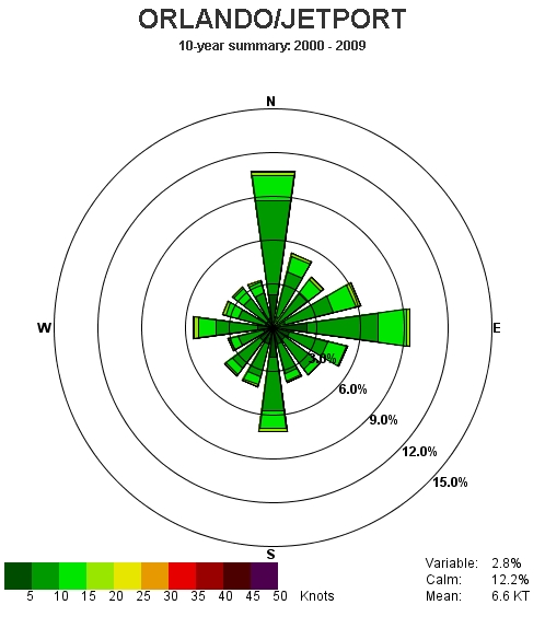
Diagram angin mawar (wind rose) adalah alat visual klasik untuk merangkum distribusi arah dan kecepatan angin di suatu lokasi selama satu periode waktu. Setiap "kelopak" (petal) menunjuk ke arah asal angin — bukan ke mana angin bertiup — dan panjangnya mencerminkan persentase waktu angin berhembus dari arah tersebut. Pita warna di dalam kelopak menunjukkan kontribusi tiap kelas kecepatan: kelopak yang panjang dengan pita warna gelap menandakan angin kuat yang sering datang dari arah tersebut.
Untuk Indonesia, wind rose punya nilai klimatologis yang tinggi. Monsun mendominasi pola angin permukaan sepanjang tahun: angin baratan (dari barat dan barat laut) berhembus saat musim hujan sekitar Oktober–April, sementara angin timuran (dari timur dan tenggara) mendominasi musim kemarau sekitar Mei–September. Pada wind rose tahunan, kedua rezim ini muncul sebagai dua kluster kelopak yang saling berhadapan — pola bimodal yang khas dari iklim monsun. Seorang praktisi yang melihat wind rose di satu titik Laut Jawa seketika bisa mengidentifikasi dominansi Angin Baratan versus Angin Timuran tanpa harus membaca tabel.
Tutorial ini membangun wind rose dari awal menggunakan data ERA5 tahun 2024 untuk satu titik representatif di Laut Jawa. Kita mulai dari mengunduh komponen angin \(u_{10}\) dan \(v_{10}\), lalu menghitung kecepatan skalar dan arah meteorologis, membin ke 16 sektor arah dan 5 kelas kecepatan, dan merender polar bar chart dengan matplotlib.
Data ERA5 untuk Komponen Angin 10 Meter
ERA5 menyediakan dua variabel angin permukaan: komponen \(u\) (ke timur, positif = eastward) dan komponen \(v\) (ke utara, positif = northward), keduanya di ketinggian 10 m atas permukaan dalam satuan m s\(^{-1}\). Resolusi horizontal ERA5 adalah \(0{,}25° \times 0{,}25°\) — sekitar 28 km — dengan cakupan waktu dari Januari 1940 hingga beberapa hari terakhir, diperbarui dengan latensi sekitar 5 hari.
Kita ambil data 6-hourly (4 timestep/hari) sepanjang 2024 untuk domain Indonesia: 6°N–11°S, 95°E–141°E. Untuk tutorial ini kita pilih satu titik representatif di Laut Jawa dekat Jakarta (\(-6{,}0°\)S, \(107{,}0°\)E) — kawasan maritim yang merasakan langsung pergantian monsun. Ini memberikan 1464 sampel sepanjang tahun.
Daftar akun di cds.climate.copernicus.eu dan konfigurasikan ~/.cdsapirc sebelum menjalankan snippet berikut. Cache guard memastikan download hanya terjadi sekali — jika file sudah ada di direktori kerja, baris cdsapi dilewati.
import os, cdsapi, xarray as xr, numpy as np

REQ = {
    "u10": ("era5_u10_indonesia_2024_6h.nc", "10m_u_component_of_wind"),
    "v10": ("era5_v10_indonesia_2024_6h.nc", "10m_v_component_of_wind"),
}
for short, (out, var) in REQ.items():
    if not os.path.exists(out):
        c = cdsapi.Client(quiet=True)
        c.retrieve("reanalysis-era5-single-levels", {
            "product_type": "reanalysis",
            "variable": [var],
            "year": "2024",
            "month": [f"{m:02d}" for m in range(1, 13)],
            "day":   [f"{d:02d}" for d in range(1, 32)],
            "time":  ["00:00", "06:00", "12:00", "18:00"],
            "area":  [6, 95, -11, 141],
            "format": "netcdf",
        }, out)

LAT, LON = -6.0, 107.0   # Laut Jawa dekat Jakarta
u10 = xr.open_dataset("era5_u10_indonesia_2024_6h.nc")["u10"].sel(
    latitude=LAT, longitude=LON, method="nearest")
v10 = xr.open_dataset("era5_v10_indonesia_2024_6h.nc")["v10"].sel(
    latitude=LAT, longitude=LON, method="nearest")
print("Titik terpilih:", float(u10.latitude), "lintang,", float(u10.longitude), "bujur")
print("Jumlah sampel waktu:", u10.valid_time.size)
print("u10 contoh:", float(u10.isel(valid_time=0)), "m/s | v10 contoh:",
      float(v10.isel(valid_time=0)), "m/s")
Titik terpilih: -6.0 lintang, 107.0 bujur
Jumlah sampel waktu: 1464
u10 contoh: 0.199981689453125 m/s | v10 contoh: 0.7613983154296875 m/s
Output di atas mengonfirmasi koordinat titik grid terdekat yang dipilih xarray dan jumlah timestep sepanjang 2024. Variabel u10 dan v10 kini tersimpan sebagai DataArray 1-D dengan koordinat valid_time — siap untuk kalkulasi.
Menghitung Kecepatan dan Arah Angin
Langkah berikutnya adalah mengubah komponen vektor \((u, v)\) menjadi dua besaran skalar: kecepatan dan arah. Kecepatan angin adalah norma vektor:
$$|\mathbf{V}| = \sqrt{u^2 + v^2}$$
Untuk arah, kita gunakan konvensi meteorologis — yaitu arah FROM-direction dalam derajat searah jarum jam dari utara sejati (0° = Utara, 90° = Timur, 180° = Selatan, 270° = Barat). Formula yang direkomendasikan ECMWF adalah:
$$\Phi = \left(180 + \frac{180}{\pi} \cdot \text{atan2}(u,\, v)\right) \bmod 360$$
Perhatikan urutan argumen: \(\text{atan2}(u, v)\) — bukan \((v, u)\). Ini berbeda dari konvensi trigonometri standar. Dalam NumPy ini menjadi np.arctan2(u, v). Sebagai sanity check: angin murni ke timur (\(u=1, v=0\)) berarti angin datang dari barat, sehingga hasilnya harus \(270°\).
spd  = np.sqrt(u10.values**2 + v10.values**2)
wdir = (180 + np.degrees(np.arctan2(u10.values, v10.values))) % 360

print(f"Kecepatan rata-rata : {spd.mean():.2f} m/s")
print(f"Kecepatan maksimum  : {spd.max():.2f} m/s")
print(f"Contoh arah 5 pertama (dari): {wdir[:5].round(1)} derajat")

# Verifikasi: angin murni ke timur (u=1, v=0) → dari barat → harus 270°
test = (180 + np.degrees(np.arctan2(1.0, 0.0))) % 360
print(f"Verifikasi u=1, v=0 → {test:.0f}° (diharapkan 270°)")
Kecepatan rata-rata : 2.77 m/s
Kecepatan maksimum  : 7.79 m/s
Contoh arah 5 pertama (dari): [194.7 327.  256.9 119.6 155.4] derajat
Verifikasi u=1, v=0 → 270° (diharapkan 270°)
Baris terakhir memverifikasi formula: angin murni ke timur benar-benar menghasilkan \(270°\). Di titik Laut Jawa ini, kecepatan rata-rata tahunan sekitar 2,8 m/s dengan puncak mendekati 8 m/s — angin permukaan di perairan dangkal ekuatorial memang cenderung moderat sepanjang tahun. Array spd dan wdir tersimpan sebagai globals dan langsung dipakai di snippet berikutnya.
Binning Sektor dan Kelas Kecepatan
Wind rose standar membagi 360° menjadi 16 sektor, masing-masing selebar \(22{,}5°\), dengan label kompas N, NNE, NE, ENE, ..., NNW. Kelas kecepatan yang kita gunakan: \([0\text{–}2,\ 2\text{–}4,\ 4\text{–}6,\ 6\text{–}8,\ {>}8]\) m/s — pilihan umum untuk angin laut di Indonesia.
Ada satu detail penting untuk sektor Utara: arah \(0°\) (Utara) harus berada di tengah sektor, bukan di tepinya. Artinya sektor N mencakup \([348{,}75°,\ 11{,}25°)\). Caranya: geser setiap arah sebesar \(+11{,}25°\), lalu bagi dengan \(22{,}5°\) dan ambil floor, kemudian modulo 16 agar nilai \(\geq 16\) wrap ke 0. Ini menangani wrap-around tanpa perlu logika kondisional khusus.
import pandas as pd

N_SECTORS  = 16
SECTOR_DEG = 360 / N_SECTORS        # 22.5°
speed_edges = [0, 2, 4, 6, 8, np.inf]
class_labels = ["0–2", "2–4", "4–6", "6–8", ">8"]

# Bin arah: geser +11.25° supaya sektor N mencakup [348.75°, 11.25°)
sector_idx = np.floor(((wdir + 11.25) % 360) / SECTOR_DEG).astype(int) % N_SECTORS
speed_idx  = np.digitize(spd, speed_edges[1:-1])   # 0..4

# Tabel frekuensi 16×5 (persentase)
freq = np.zeros((N_SECTORS, len(class_labels)))
for s, v in zip(sector_idx, speed_idx):
    freq[s, v] += 1
freq = freq / len(spd) * 100

compass = ["N","NNE","NE","ENE","E","ESE","SE","SSE",
           "S","SSW","SW","WSW","W","WNW","NW","NNW"]
df = pd.DataFrame(freq, index=compass, columns=class_labels)
df["Total"] = df.sum(axis=1)
print(df.round(2).to_string())
print(f"\nTotal semua sektor: {df['Total'].sum():.1f}%")

# Simpan sudut tengah tiap sektor (radian) untuk snippet-4
sector_centers = np.radians(np.arange(N_SECTORS) * SECTOR_DEG)
      0–2   2–4   4–6   6–8   >8  Total
N    0.75  1.91  0.07  0.00  0.0   2.73
NNE  1.37  3.69  0.07  0.00  0.0   5.12
NE   1.16  5.46  0.96  0.07  0.0   7.65
ENE  1.30  4.71  2.25  0.07  0.0   8.33
E    1.98  5.12  0.89  0.00  0.0   7.99
ESE  3.55  4.99  0.55  0.00  0.0   9.08
SE   4.64  5.60  0.14  0.00  0.0  10.38
SSE  4.99  1.30  0.00  0.00  0.0   6.28
S    2.94  0.96  0.00  0.00  0.0   3.89
SSW  2.32  0.48  0.00  0.00  0.0   2.80
SW   1.64  1.23  0.34  0.00  0.0   3.21
WSW  1.30  3.48  4.10  0.48  0.0   9.36
W    1.30  3.28  3.62  0.68  0.0   8.88
WNW  0.96  2.80  2.25  0.34  0.0   6.35
NW   1.50  2.39  1.23  0.20  0.0   5.33
NNW  1.16  1.37  0.07  0.00  0.0   2.60

Total semua sektor: 100.0%
Tabel di atas menampilkan persentase waktu angin berhembus dari setiap kombinasi arah dan kelas kecepatan. Kolom "Total" yang dijumlahkan harus mendekati \(100{,}0\%\) — konfirmasi bahwa semua sampel terbagi ke dalam satu sektor tanpa ada yang terlewat.
Membuat Diagram Angin Mawar dengan Matplotlib
Semua bahan sudah tersedia: freq (array 16×5 frekuensi persen), sector_centers (sudut radian tiap sektor), dan class_labels. Kita render polar bar chart dengan matplotlib, di mana sumbu-\(\theta\) mewakili arah kompas dan tinggi bar mewakili frekuensi (%). Bar disusun bertumpuk (stacked) per kelas kecepatan sehingga tinggi total satu kelopak = total frekuensi dari arah tersebut.
Dua konfigurasi kritis pada polar axes: set_theta_zero_location("N") meletakkan \(\theta = 0\) di atas (Utara), dan set_theta_direction(-1) membuat sudut bertambah searah jarum jam — persis konvensi kompas. Tanpa keduanya, Utara akan muncul di kanan dan rotasi berjalan berlawanan arah.
import matplotlib
matplotlib.use("Agg")
import matplotlib.pyplot as plt

colors = ["#2166ac", "#74add1", "#ffffbf", "#f46d43", "#a50026"]
width  = 2 * np.pi / N_SECTORS * 0.9   # sedikit celah antar bar

fig, ax = plt.subplots(figsize=(9, 9), subplot_kw={"projection": "polar"})
ax.set_theta_zero_location("N")
ax.set_theta_direction(-1)

bottoms = np.zeros(N_SECTORS)
for i, (label, color) in enumerate(zip(class_labels, colors)):
    ax.bar(sector_centers, freq[:, i], width=width, bottom=bottoms,
           color=color, label=f"{label} m/s", edgecolor="white", linewidth=0.4)
    bottoms += freq[:, i]

compass_labels = ["U", "NNE", "TL", "ENE", "T", "ESE", "TG", "SSE",
                  "S", "SSW", "BD", "WSW", "B", "WNW", "BL", "NNW"]
ax.set_xticks(sector_centers)
ax.set_xticklabels(compass_labels, fontsize=9)
ax.set_title(
    "Diagram Angin Mawar — Laut Jawa (2024)\nERA5 Angin 10 m, 6°S 107°E",
    pad=22, fontsize=13, fontweight="bold")
ax.set_ylabel("Frekuensi (%)", labelpad=30, fontsize=9)
ax.yaxis.grid(True, linestyle="--", alpha=0.5)
ax.legend(loc="upper left", bbox_to_anchor=(-0.18, 1.05),
          title="Kelas Kecepatan", fontsize=9, title_fontsize=10)

fig.savefig("wind_rose.png", dpi=120, bbox_inches="tight")
print("Wind rose tersimpan.")

Diagram di atas adalah wind rose tahunan di Laut Jawa berdasarkan data ERA5 2024. Kelopak-kelopak yang menonjol menandai arah dominan angin di lokasi tersebut, dan pita warna di dalamnya menunjukkan sebaran kelas kecepatan.
Interpretasi Monsun Indonesia dan Pola Tahunan
Wind rose tahunan di Laut Jawa mencerminkan dua rezim monsun yang bergantian. Selama musim hujan (sekitar Oktober–April), angin baratan dari arah barat hingga barat laut mendominasi — ini adalah Angin Baratan (Asian monsoon) yang membawa kelembapan dari Samudra Hindia dan Laut China Selatan. Selama musim kemarau (sekitar Mei–September), arah berbalik: angin timuran dari timur hingga tenggara (Angin Timuran, Australian monsoon) membawa udara lebih kering dari benua Australia.
Hasilnya adalah pola bimodal — dua kluster kelopak yang saling berhadapan di wind rose — yang langsung terbaca sebagai sidik jari iklim monsun. BMKG mencatat bahwa perpindahan dari Angin Baratan ke Angin Timuran menandai onset musim kemarau di 699 zona musim (ZOM) Indonesia, dan timing transisi ini dipengaruhi oleh ENSO dan IOD dari tahun ke tahun.
Untuk eksplorasi lebih lanjut, coba buat wind rose terpisah untuk musim hujan (Desember–Februari) dan musim kemarau (Juni–Agustus) — perbedaannya jauh lebih dramatis dan secara visual langsung menggambarkan pembalikan monsun. Kita juga bisa mereplikasi analisis ini ke beberapa titik sekaligus untuk memetakan variasi spasial pola angin permukaan di seluruh kepulauan.
Eksplorasi artikel meteorologi lainnya di meteo.my.id. Kunjungi halaman utama untuk arsip lengkapnya.
Referensi
- ERA5: How to calculate wind speed and wind direction from u and v components of the wind — Formula resmi ECMWF untuk menghitung kecepatan dan arah angin meteorologis dari komponen u dan v ERA5, termasuk peringatan urutan argumen atan2.
- ERA5: data documentation — Dokumentasi lengkap variabel ERA5 single-levels, resolusi \(0{,}25°\), dan cara akses via Copernicus Climate Data Store.
- How to Read a Wind Rose — Panduan EPA tentang cara membaca diagram angin mawar: arti kelopak, pita warna, dan interpretasi klimatologis.
- BMKG: Musim Kemarau 2026 Datang Lebih Awal, Puncak Terjadi Agustus Mendatang — Siaran pers BMKG tentang prediksi onset musim kemarau 2026 dan transisi monsun di 699 ZOM Indonesia.


